Linear Algebra with Python and NumPy (I)
Linear Algebra with Python and NumPy (I)
Recently, I've learned to use Python to create Blender addons, which made me appreciate the elegance and flexibility of this scripting language. Also, there are lots of Python based tools like Jupyter Notebook, which I'm just using to write this post. Or Spyder, the complete IDE for scientific computing, which is quite similar to the well known Matlab.
Although as a former user of Matlab/Octave language, I've faced few differences related to algebraic structures. It's known that Matlab is probably the most intuitive language when it comes to numerical computing, but compared to Python it has other shortcomings. Besides, when the final code for my usage is going to be Python, it seems reasonable to use Python from the start of development process, rather than develop an algorithm in Matlab and then translate it into Python. Therefore, this post is mainly focused on the differences you need to keep in mind when coming to Python from Matlab.

So, lets get started with Python computing :)
First, we need to import the package NumPy, which is the library enabling all the fun with algebraic structures.
from numpy import *
1 Complex Numbers
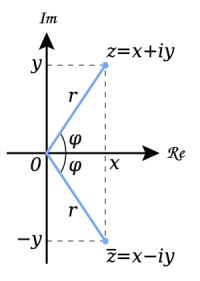
A complex number is a number of the form $z = x + jy$, where $x$ and $y$ are real numbers and $j$ is the imaginary unit, satisfying $j^2 = −1$. Note that the imaginary unit, often denoted as $i$, is denoted as $j$ in Python.
The set $\mathbb{C}$ of all complex numbers can be actually defined as the set of ordered pairs of real numbers $\{(x,y) \mid x,y\in\mathbb{R} \}$ that satisfies the following operations
- addition: $(a,b)+(c,d) = (a+c,b+d)$
- multiplication: $(a,b)\cdot(c,d) = (ac-bd,ad+bc)$
Then, it's just a matter of notation to express a complex number as $(x, y)$ or as $x + jy$.
When we have a complex number $z\in\mathbb{C}$, we can denote its real and imaginary part as
$$ x = \Re(z), \quad y = \Im(z). $$
The complex conjugate of the complex number $z = x + jy$ is denoted by either $\bar{z}$ or $z^*$ and defined as
$$\bar{z} = x − jy .$$
The absolute value (or modulus or magnitude) of a complex number $z = x + jy$ is
$$ | z | = \sqrt{x^2+y^2} = \sqrt{z \bar{z}} .$$
z = 3 + 4j                  # Define a complex number z
print('z =', z)
print('Re(z) =', real(z))   # Get real part of z
print('Im(z) =', imag(z))   # Get imaginary part of z
print('|z| =', abs(z))      # Get absolute value of z
Note that to obtain $j=\sqrt{-1}$ we must write the argument of sqrt function as a complex number (even if has zero imaginary part), otherwise Python tries to compute sqrt on real numbers and throws an error.
z = sqrt(-1+0j)
print('sqrt(-1) =', z)
2 Vectors and Matrices
Using NumPy we can define vectors and matrices, both real or complex. Although, in contrast to Matlab, where matrix is the default type, in Python we need to define vectors and matrices as array or matrix type.
a = array([10,20,30])   # Define a vector of size 3 using type 'array'
print(a)
print(a.shape)          # Size/shape of vector
b = matrix('10 20 30')  # Define a vector of size 3 using type 'matrix'
print(b)
print(b.shape)          # Size/shape of vector
c = linspace(10,20,6)   # Define vector as 6 values evenly spaced from 10 to 20
print(c)
Note that matrix and array elements in Python are indexed from 0, in contrast to Matlab where indexing starts from 1.
print(c[:])     # Get all elements
print(c[0])     # The first element
print(c[-1])    # The last element
print(c[:3])    # The first 3 elements
print(c[-3:])   # The last 3 elemnets
print(c[2:4])   # 2:4 selects elements of indexes 2 and 3
Euclidean norm of vector is returned by method numpy.linalg.norm
norm = linalg.norm(a)      # Euclidean norm of vector a
print('a =', a)
print('norm(a) =', norm)

x = a/linalg.norm(a)       # Make normalized/unit vector from a
print('\nx =', x)
print('norm(x) =', linalg.norm(x))
Transposition of vectors is not so intuitive as in Matlab, especially if a vector is defined as 1D array and you cannot distinguish between row and column vector. However, using the keyword newaxis it's possible to shape the vector into 2D array (as matrix of size $1 \times n$ or $n \times 1$), where transposition makes sense and can be obtained by attribute .T.
a = array([10,20,30])
x = a[:,newaxis]  # Make column vector from vector a (defined as array)
print(x)
print(x.shape)    # Now size of column vector is 3x1
print(x.T)        # Make row vector by transpostion of column vector
If a vector was defined as 2D array of type matrix, transportation is not a problem.
b = matrix('10 20 30')
x = b.T           # Make column vector from vector b (defined as matrix)
print(x)
print(x.shape)    # Now size of column vector is 3x1
print(x.T)        # Make row vector by transpostion of column vector
Matrices can be defined as 2D arrays of type array or matrix (there is no problem with transposition with any type).
A = array([[11,12,13], [21,22,23], [31,32,33]])  # Define matrix of size 3x3 as 2D 'array-type'
print(A)
print(A.shape)
B = matrix('11 12 13; 21 22 23; 31 32 33')  # Define matrix of size 3x3 as 'matrix-type'
print(B)
print(B.shape)
print(B[0,1])    # Get matrix element at row 0, column 1
print(B[0,:])    # Get 1st row of matrix (A[0] returns also 1st row)
print(B[:,0])    # Get 1st column of matrix
print(A[:,0])   # Note that column from 'array-type' matrix is returned as 1D array
print(B[:,0])   # Column from 'matrix-type' matrix is returned as true column as expected
NumPy can generate some essential matrices exactly like Matlab.
print('3x3 Matrix full of zeros:')
print(zeros([3,3]))

print('\n3x3 Matrix full of ones:')
print(ones([3,3]))

print('\n3x3 identity matrix:')
print(eye(3))

print('\n3x3 diagonal matrix:')
x = array([1.,2.,3.])
print(diag(x))

print('\n3x3 random matrix:')
print(random.rand(3,3))
For merging matrices or vectors methods numpy.hstack and numpy.vstack can be used.
print(vstack([ A, ones([1,3]) ]))  # Add row vector to matrix
print(hstack([ A, ones([3,1]) ]))  # Add column vector to matrix
print(hstack([ A, eye(3) ]))       # Merge two matrices horizontally
3 Operations with Matrices
Matrix transposition is obtained by attribute .T
X = ones([2,5])  # Generate 2x5 matrix full of ones
print('Matrix X of size', X.shape)
print(X)

Y = X.T          # Obtain transpose of matrix X
print('\nMatrix Y=X.T of size', Y.shape)
print(Y)
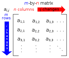
Hermitian transpose (or conjugate transpose) of complex matrix $\mathbf{A}\in\mathbb{C}^{m\times n}$ is obtained by taking the transpose of $\mathbf{A}$ and then taking the complex conjugate of each element. Note that for real matrices Hermitian transpose and plain transpose does not differ. In NumPy this kind of transposition is obtained by attribute .H (exists only for matrix type).
X = matrix((3+4j)*ones([2,5]))  # Generate matrix full of complex elements 3+4j
print('Matrix X of size', X.shape)
print(X)

Y = X.H                         # Obtain Hermitian transpose of matrix X
print('\nMatrix Y=X.H of size', Y.shape)
print(Y)
Matrix multiplication must be executed by method for dot product numpy.dot. Operator * produces only element-wise multiplication in Python.
print('Matrix A:')
print(A)

print('\nMatrix B:')
B = ones([3,3])
print(B)

print('\nElement-wise multiplication A*B:')
print(A*B)

print('\nMatrix multiplication A by B:')
print(dot(A,B))

print('\nMatrix multiplication B by A:')
print(dot(B,A))
There are also methods for essential matrix features like Frobenius norm, rank or determinant.
print('Matrix A of size', A.shape)
print(A)

# Frobenius norm of matrix
print('\nFrobenius norm: ||A|| =', linalg.norm(A))

# Rank of matrix
print('rank(A) =', linalg.matrix_rank(A))

# Determinant of matrix
print('det(A) =',  linalg.det(A))
In example above, note that the matrix $\mathbf{A}$ is a singular matrix, because its rank is lower than number of its rows, thus also its detemninat is zero.
4 Conclusion
As we can see from this article, Python and NumPy package can be used to perform all the usual matrix manipulations. There are only few things one need to keep in mind when writing Python code. For example, operator * applied to matrices doesn't produce matrix product, but only element-wise multiplication. Or vectors, many methods return them just as 1D array, so we need to convert them into 2D array or matrix type first, to be able to distinguish between row and column vector.
Comments
Comments powered by Disqus